Calculations sheet
The workbooks and a pdf-version of this user manual can be downloaded from here.
The Calculations sheet of Meta-Essentials contains all calculations underlying the output in the other sheets. It can be accessed by clicking on the regarding tab, as shown in Figure 17. It is a rather extensive sheet in which different parts are clearly indicated by a header. This sheet has no other function than documenting the intermediary outputs of an analysis, or equivalently, the transformations between input and output. Because reading this sheet is not necessary for running a meta-analysis (or for other types of analysis in Meta-Essentials) and because column names are (hopefully) self-explanatory, this sheet will be discussed only very briefly in this manual.

Figure 30: The tab to access the Publication Bias Analysis sheet of Meta-Essentials
Forest Plot
The first part contains the necessary calculations to construct the Forest Plot sheet (see Figure 31 for an example). The first two columns give ranks for the presentation functions ‘Sort By’ and ‘Order’ on the Input sheet. Effect sizes, variances, standard errors, the weights, in both fixed effect and random effects models, are provided along with the confidence interval limits. Finally, the relative weight the study receives in the model is given (based on the choice between fixed effect and random effects). The second table repeats the estimates of effects size as well as the lengths of the confidence interval bars for plotting purposes. On the right side the same is done for the combined effect size. Note that cells showing “#N/A” are meant to show these errors since it is the only way to let Excel ignore them when making the plots, unfortunately.
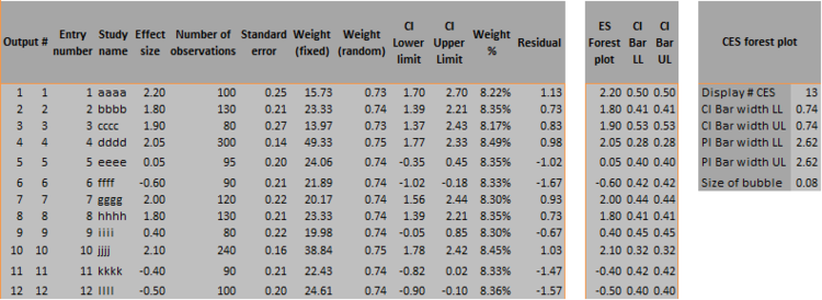
Figure 31: Example of Forest Plot part of the Calculations sheet
Subgroup Analysis
The subgroup analysis section of the calculations sheet contains the necessary calculations to construct the Subgroup Analysis sheet. It begins with repeating the information from the input section (see Figure 32 for an example). The first section, to the left, gives information per study. The ‘Display # studies’ as well as the information in the second table of the following picture are for plotting purposes. The weights in a random model (if that was chosen in the Subgroup Analysis sheet) depend on subgroup estimates of heterogeneity, either separate per subgroup or pooled over subgroups, as specified in the Subgroup Analysis sheet.
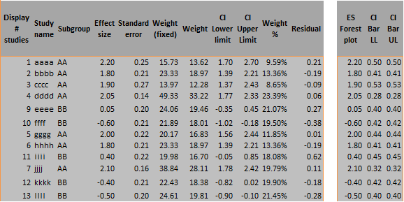
Figure 32: Example of first part of Subgroup Analysis part of the Calculations sheet Subgroup Analysis
The second section refers to subgroups and starts with a display number for plotting purposes (see Figure 33 for an example). It gives the name of the subgroup, the subgroup number, and the number of studies in the subgroups followed by heterogeneity measures and subgroup combined effect sizes estimates with standard errors, confidence and prediction interval limits and finishes with weights for fixed effect and random effects models.

Figure 33: Example of second part of Subgroup Analysis part of the Calculations sheet
The third and final section of the Subgroup Analysis part of the Calculation sheet contains information for the combined effect size as well as heterogeneity measures (see Figure 34 for an example). Below these estimates the between and within subgroup weighting methods input options are given in text (for reference purposes).
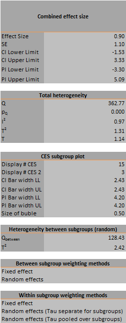
Figure 34: Example of third part of Subgroup Analysis part of the Calculations sheet
Moderator Analysis
This part of the Calculations sheet contains the necessary calculations for the Moderator Analysis sheet (see Figure 35 for an example). The first table repeats information from the input section (‘Moderator’ and ‘Effect Size’) for plotting purposes. The first table furthermore contains information from a fixed effect model, the second table from a random effects model and the third for the combined effect size and heterogeneity measures in a fixed effect model. Below the third table the regression line is given for plotting purposes.
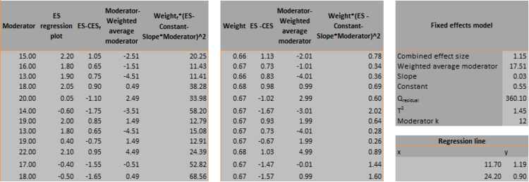
Figure 35: Example of Moderator Analysis part of the Calculations sheet
Publication Bias Analysis
This part of the Calculations sheet contains the necessary calculations for the Publication Bias Analysis sheet and is divided a similar fashion as the regarding sheet. That is, the sheet is divided in sections for each procedure or statistic regarding publication bias analysis.
Funnel plot
The funnel plot section contains information for weighting, ranks for the trim and fill plot (discussed later) in the first table and gives estimates of the funnel lines, confidence and prediction interval bars of observed and adjusted combined effect sizes for plotting purposes in the rest of the tables (see Figure 36 for an example).
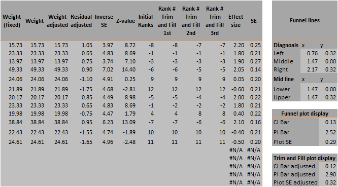
Figure 36: Example of Funnel Plot part of the Calculations sheet
Trim and fill plot
The first table in the trim and fill plot section gives the differences between the study’s effect size and the combined effect size (denoted by Xi), its absolute and the weight the study receives (see Figure 37 for an example). This is given three times because of the before mentioned three iterations. The ranks in the funnel plot section are derived by ranking the absolutes of Xi and multiplying by minus one if Xi is negative (for pragmatic reasons these are included in the Funnel Plot part, shown before in Figure 36). The second part gives the combined effect size iterations with the combined effect size, heterogeneity and estimated number of missing studies per iteration.
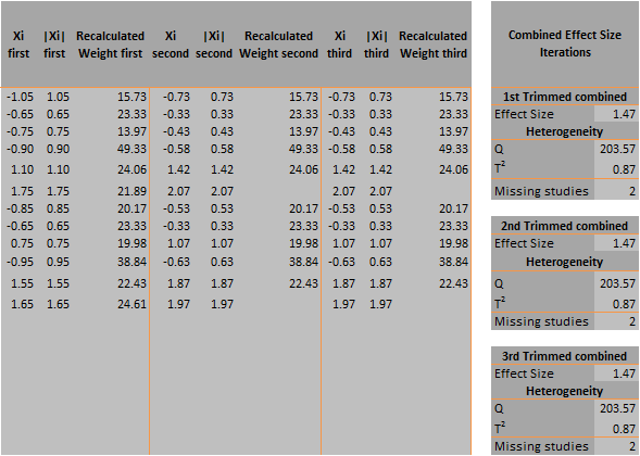
Figure 37: Example of first and second part of Funnel Plot part of the Calculations sheet
The third part contains information for the imputed data points, the estimated effect size and standard error and repeats that information in the fourth table for plotting purposes (see Figure 38 for an example). Note that we usually base the examples in this user manual on the fictious example data from Workbook 1, ‘Effect size data.xlsx’. However, since there are no imputed studies based on these data, we use another fictious example for Figure 38.
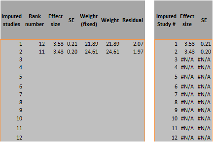
Figure 38: Example of third and fourth part of Trim and Fill part of the Calculations sheet
Egger regression
The calculations for the Egger regression are mostly executed directly on the Publication Bias Analysis sheet, except for some estimates needed for the calculations of the standard errors of the regression estimates (see Figure 39 for an example).

Figure 39: Example of Egger Regression part of the Calculations sheet
Begg & Mazumdar rank correlation test
For the Begg & Mazumdar rank correlation test, an adjusted effect size and variance are first derived, followed by their respective ranks, all denoted with a star (*) to indicate that they are adjusted estimates (see Figure 40 for an example). Under x, the count of concordant ranks is given and under y, the count of discordant ranks is given. The remainder of the calculations is executed directly on the Publication Bias Analysis sheet.
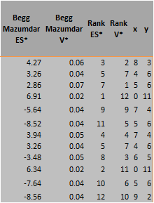
Figure 40: Example of Begg & Mazumdar Rank Correlation part of the Calculations sheet
Standardized Residual Histogram
The calculations for the standardized residual histogram consist of one table below for the calculation of the width of the bins and a table on top with the lower, middle and upper values of the bins (see Figure 41 for an example).
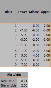
Figure 41: Example of Standardized Residual Histogram part of the Calculations sheet
Galbraith plot
For the Galbraith plot, the calculations section contains the inverse standard error and z-score for plotting purposes (see Figure 42 for an example). The second table contains information for the regression lines in the plot.
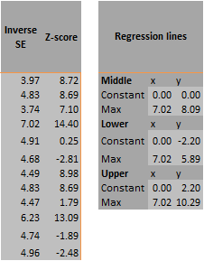
Figure 42: Example of Galbraith Plot part of the Calculations sheet
Normal Quantile Plot
The calculations for the normal quantile plot contain information on the ranks, the normal and sample quantile for plotting purposes and some information for the calculation of the standard error of the regression estimates (see Figure 43 for an example). The second table is used for plotting the regression line.
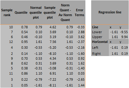
Figure 43: Example of Normal Quantile Plot part of the Calculations sheet
Failsafe-N tests
For the Failsafe numbers, the z-score, its p-value and a log-value of the p-value are given (see Figure 44 for an example). Note that because Excel cannot cope with more than 15 digits in its calculations ‘under the hood’, it will round the very small p-values to zero. Therefore, the natural logarithm of that value would give an error since the natural logarithm of zero is undefined. To overcome this problem Meta-Essentials automatically replaces p-values of zero with 10-306, which natural logarithmic is -704.59, shown in several instances in the example.
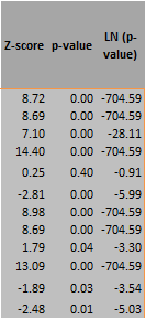
Figure 44: Example of Failsafe-N part of the Calculations sheet


