Subgroup analysis

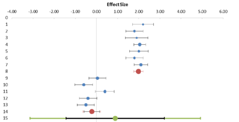
As previously discussed, the forest plot in Figure 1 suggests that there are two subgroups in the domain that have a different “true” effect size. If this was a study of the effect of an intervention, it could be that we are dealing here with results from studies in different countries. It is possible to explore a hypothesis about a difference in effect between subgroups. This is, however, only possible for known characteristics of the populations that were studied. These characteristics must have been coded and entered on the Input sheet of the software. Figure 5 is an example of a forest plot on the Subgroup Analysis sheet for the same studies as have been discussed before (Figure 1). It is a bit misleading in the sense that the neat separation between the two subgroups in this plot is the result of how we have set up the example. In this fictitious example, code AA is assigned to all studies with an effect size around 2.0 and code BB has been assigned to the other studies. In actual practice, it is rare to find the effects observed in subgroups so clearly different in every single study. If study 4, for instance, would have been a study of subgroup BB, then the results would have been very different for subgroup BB.

Note that the weighted average effect (0.89) in Figure 5 is different from the one in Figure 1 (1.07) and that both the confidence interval and the prediction interval are larger. These differences between the results in these two plots can be explained by the fact that the average effect and its intervals in Figure 5 are calculated from the subgroup effects (N=2) and those in Figure 1 from the effects observed in the original studies (N=14). Therefore, it is not recommended to use information about the combined effect and its intervals from the subgroup analysis!

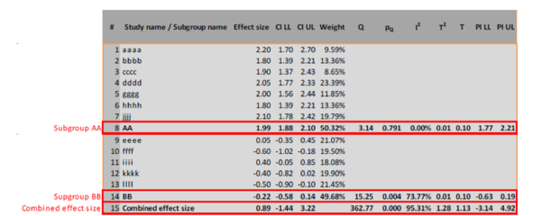
For the interpretation of the results within a subgroup, the same principles and caveats apply as were discussed for forest plots and meta-analytic results in general. Similarly, the meta-analyst should first interpret Information about heterogeneity. In Meta-Essentials, heterogeneity parameters for each subgroup are computed and presented (see Figure 6). 

Whereas, in this example, it appeared to be erroneous to assume that the total set of studies (Figure 1) can be seen as studies of one (homogeneous) population, it appears to be possible to treat at least one of the subgroups as a homogeneous population. Figure 6 presents, among other things, the four heterogeneity parameters for each of the two subgroups. I² for subgroup AA is 0%, indicating that all studies in this subgroup have produced an estimate of the same “true” effect size in a homogeneous population (AA). The estimate of the effect is 1.99 (95%CI 1.88-2.10). In this subgroup, the information about the prediction interval (1.77-2.21) can be ignored. I² for subgroup BB is almost 74%, indicating that this subgroup is very heterogeneous and hence cannot be meta-analysed as if it is one single population. This implies that it is not useful to interpret the combined effect in subgroup BB, and hence we should focus on the prediction interval (from -0.63 to 0.19) rather than on the estimate and its confidence interval.

Note that Meta-Essentials does not give statistical information about the size of the difference between the average subgroup effects. Obviously, this difference can easily be calculated by the researcher from the information in Figure 6 (it is 2.21), but it is not recommended to do so for the heterogeneity of subgroup BB. There is no meaningful average effect in this subgroup and hence there is no value that can be compared with the effect in subgroup AA. The inclusion of the Subgroup analysis in Meta-Essentials, thus, is not primarily aimed at supporting an analysis of the differences between subgroups. It is rather aimed at supporting the identification of subgroups that might be homogeneous enough to allow estimation of a combined effect in that subgroup (as subgroup AA in the example).

If it assumed that there is no relevant selection bias in the set of studies from subgroup AA (which is a rather problematic assumption that can only be proven to be correct after inclusion of many more studies), then the average effect size might be interpreted as an estimate of the “true” effect in AA. In more practical terms, if this is a meta-analysis of the effects of an intervention on an educational outcome, then the results of the combined meta-analysis (as presented on the forest plot sheet; Figure 1) cannot be used as evidence for its effectiveness or lack of effectiveness. However, the results of the subgroup analysis (Figure 6) indicate that the treatment is effective in AA (e.g., in the United Kingdom) with an effect size around 2.0.